Microsoft Excel – Tech Savvy Life

How to Format a Zip Code in Microsoft Excel

When entering numbers into Microsoft Excel, leading zeros are removed by default. This can be problematic for ZIP codes, phone numbers, credit/debit card numbers and IDs that you type into a cell. We are going to explore some options on fixing this Excel behavior.

If you want to keep a leading zero on the fly, you can enter an apostrophe (‘) before you enter the number that begins with zero. Excel treats the number as a text field. The apostrophe (‘) is not displayed and calculations will still work. But who wants to do this every time, there has to be a better way.

This is for Excel for Office 365 Windows and Mac versions. Other versions of Excel will be similar.

Create the Excel Sheet

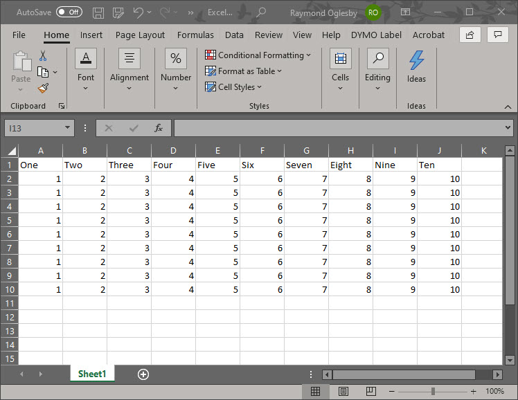
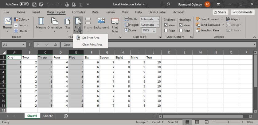
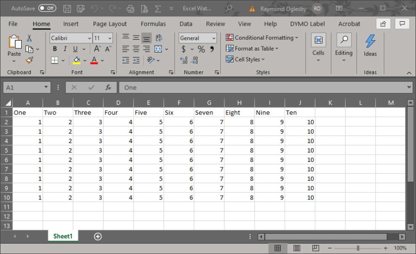
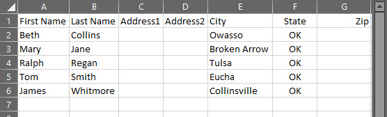
Create a simple Excel sheet like the example below:

Zip Code Format 1 — Excel Sheet for Zip Codes

Setup the Zip Code Format

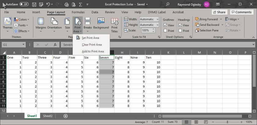
Select a cell or range of cells to format; in my case G2 thru G6
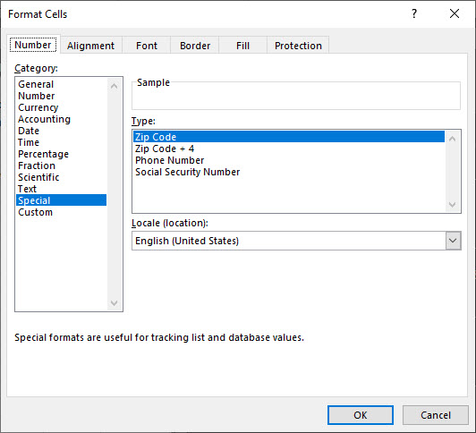
Click “Ctrl+1” to load Format Cells dialog. Also, you can right click and select Format Cells.
Select the Number tab
Select Custom from the Category list
In the Type box, type in 00000 for a five digit zip code or 00000-0000 for a nine digit zip code. This allows leading zeros to be placed in the cell, you only have to enter the Zip code numbers. This is not intuitive, you think you have to select a format from the list. Refer to the following image:

Zip Code Format 3 — Setup Excel Sheet format

Using the Special Zip Code Format

You can also click Special, then select Zip Code or Zip Code + 4. In Google Sheets, this special Zip code format is not available, but you can enter the format of leading zeros. See the following example:

Zip Code Format 2 — Excel Special Zip Code format

Click OK to apply the format. The 00000 or 00000-0000 format is saved in the Type list for future use.

This will only effect Zip Codes that are entered after the format is applied.

You can also format the Zip Code as Plain Text. Anything you enter will show exactly how you typed it in text.

To do this:

Select your data range
Press “Ctrl+1” to launch the Format Cells dialog box
On the Number tab, click Text

What about Zip Codes entries that have more than 5 digits? We can use a Conditional Format in an adjacent column to flag the invalid Zip codes. I used the formula; if the length (cell reference)>5 is True then present an “Invalid Zip” message, if the expression is False, then no message is presented.

Flagging Invalid Zip Codes

Create a column adjacent to the Zip Code and label it Error Message
Set the Conditional Format for the first cell adjacent to the Zip Code. In my example, it is cell G2
Type in this formula, =IF (LEN(your cell reference)>5,”Invalid Zip”,””)
Copy this formula, then highlight a range of cells, then Paste

See the following image for the Invalid Zip message related to cell G2 and G6, both have more than 5 numbers. An important note, Excel lets you enter as many digits as allowed, there is no truncation. The template of 00000 formatting is for adding leading zeros if the number of digits is less than 5.

Zip Code Format 5 — Flagging Invalid Zip Codes screen

I Would Like to Hear from You

Please feel free to leave a comment. I would love hearing from you. Do you have a computer or smart device tech question? I will do my best to answer your inquiry. Please mention the device, app and version that you are using. To help us out, you can send screenshots of your data related to your question.

The author’s Vietnam eBook on the Battle for Tra Bong: Events and Aftermath

How to Add an Excel Watermark to Your Sheet

In Microsoft Excel, you can add a watermark, sort of, to an Excel sheet. How to do this is not intuitive. In Microsoft Word you have templates to chose from such as “Confidential” or “Do Not Copy” for a watermark.

I am going to discuss one method; adding an image background as a watermark. We are going to insert an image which could be a photo or a company logo. Let’s see how to implement this watermark.

This is for Excel for Office 365 Windows and Mac versions. Other versions of Excel will be similar.

Your Excel Sheet

Create an Excel spreadsheet or use an existing one. Refer to my newly created sheet (Sheet1) below:

Click Insert>Text>Header & Footer

xcel Watermark 3 — Inserting a Header in the middle column

Select Picture

Select Your Watermark

Select your option for inserting a picture. Refer to following screenshot

Excel Watermark 4 — Options for selecting a watermark image

Select your image
Click Insert
You will see &[Picture] in the Header.

Excel Watermark 5 — Your Header screen without the watermark being shown

View Your Watermark

Tap anywhere outside the Header to see your watermark. Refer to following screenshot for my selection of a logo:

Excel Watermark 8 — My Excel sheet with a logo as a watermark

Formatting Your Watermark

To format the image:

Tap anywhere outside the Header
Click Insert>Text>Header & Footer
Select Format Picture. You will see the following screen:

Excel Watermark 9 — Resize your watermark

From here you can resize the image

Click the Picture tab
Select the Color box and change it to the Washout option
Click OK. This allows the background image to be less intrusive.

Excel Watermark 10 — Using the Washout option

Refer below to my final capture of the watermark screen:

Excel Watermark 11 — My final screen with the watermark background dimmed in order to see the cells contents

Save your spreadsheet and close or exit Excel

For a Microsoft Word look-a-like watermark, use the WordArt feature in Excel.

I Would Like to Hear from You

Please feel free to leave a comment. I would love hearing from you. Do you have a computer or smart device tech question? I will do my best to answer your inquiry. Please mention the device, app and version that you are using. To help me out, you can send screenshots of your data related to your question.

The author’s Vietnam eBook on the Battle for Tra Bong: Events and Aftermath

Want to Print Nonadjacent Ranges in Excel?

Normally, we chose an adjacent range of cells with headers for printing in Excel. However, there are occasions we want to print nonadjacent cell ranges. There are some of us who didn’t realize you could do this in a single print area. Let’s see how this is done.

This is for Excel for Office 365 Windows and Mac versions. Other versions of Excel will be similar.

Dilbert Touching — *Copyright Scott Adams, Inc./Distributed by Universal Uclick for UFS*

First Method of Selecting Cells

One method is holding down the “Cntl” key while selecting the range of cells you want in your Print Area.

Select your first range of cells
Press and hold the “Cntl” key
Select additional ranges of cells
Release the “Cntl” key
Click the Page Layout tab
Click Print Area
Click Set Print Area. See following image for my selection of nonadjacent cells in Print Area:

Excel Print Area 1 — Selecting nonadjacent cells Print Area

Please note that each range you selected will print on a separate page in the same order that you selected regardless of cells location. Also, your current page settings will apply to all your pages. For example, you are unable to mix Landscape and Portrait printing.

Second Method of Selecting Cells

Another method is adding nonadjacent cells to an existing Print Area.

Select a range of cells you want to add to your Print Area
Click the Page Layout tab
Click Print Area
Click Add to Print Area. Refer to below image:

Excel Print Area 2 — Adding a nonadjacent cell range to Print Area

As with the first method, each range will print on a separate page in the order selected and with the same print settings.

Locate the Print Area

In the Name box to the left of the Formula bar, click it’s drop down arrow and select Print_Area. See following image:

Excel Print Area 3 — Using the Name box to show the Print Area

Alternatively, from the View tab, click Page Break Preview in the workbook Views group to see the Print Area.

Click Normal to return to default Excel view.

Two Methods on Printing Your Ranges

You may not want each nonadjacent cell range printed on a separate page. You have two options:

Move the cell ranges adjacent to each other and reset your Print Area
Before printing, select the option to Ignore Print Area. The Active Sheet is now ready for printing. Your Print Area is still saved, you are just ignoring it. Refer to following image:

Excel Print Area 4 — Ignoring the Print Area for printing

I Would Like to Hear from You

The author’s Vietnam eBook on the Battle for Tra Bong: Events and Aftermath

How to Protect an Excel Workbook, a Sheet and its Structure

Do you want to protect your Microsoft Excel workbook or a sheet in your workbook? If so, this blog post is for you. We are going to password protect a workbook, protect a sheet in a workbook and the Excel file itself.

This is for Excel for Office 365 Windows and Mac versions. Other versions of Excel will be similar.

Protect a Workbook

I recommend you start with a blank Excel workbook, just in case you forget a password. To assign a password to an Excel workbook, do the following:

Open a blank Excel workbook. For demonstration purposes, I am using an Excel workbook that contains one sheet with cell data. You can choose an existing Excel workbook if you chose. See my workbook below :

Select File>Save As

Select More options (underneath Excel Workbook drop down box)

Select the Tools drop down box
Chose General Options

Set the Password(s)

You will see notice two password boxes, one to open the workbook and one to modify the workbook

Enter one or both passwords. Make sure you write down these passwords and store them in a safe place.

You have two other options to set if you chose, Always create backup and Enable Read-only recommended. The first is self explanatory. The second option is an extra layer of protection by enabling the workbook to read-only status upon opening.

Confirm your password(s) by reentering the password(s)
Click OK
Click Save
Close or Exit Excel

Note! A user who doesn’t know the second password can open and view the data by clicking the Read Only option. This user can still modify the data, but they are unable to save their changes to the protected workbook. However, the user can save the workbook under a new name, which circumvents the protection process. Of course, password-cracking software will get you into the workbook.

Protect a Sheet

Open a blank Excel workbook. For demonstration purposes, I am using an Excel workbook that contains one sheet with cell data. You can choose an existing Excel workbook if you chose.
Select the Review tab
Click the Protect icon
Click Protect Sheet icon. Refer to following image:

Enter your password in the Password to unprotect sheet box
Click OK
In the Confirm Password dialog box, type the password again
Click OK
Save your changes
Close or Exit Excel

Tip! To remove a password, click Protect>Unprotect Sheet and enter your password. You can also select Protect Workbook icon to protect a workbook which follows.

Protect Excel Structure

Open a blank Excel workbook. For demonstration purposes, I am using an Excel workbook that contains one sheet with cell data. You can choose an existing Excel workbook if you chose.
Select the Review tab
Click the Protect icon
Click Protect Workbook icon. Refer to the following image:

Select the Windows option if you want to prevent users from moving, resizing, or closing the workbook window or hide/unhide windows

Enter your password
Click OK
In the Confirm Password dialog box, type the password again
Click OK
Save your changes
Close or Exit Excel

Protect the Excel File

To prevent users from accessing the data in your Excel file, we are going to protect the file with a password

Open a blank Excel workbook. For demonstration purposes, I am using an Excel workbook that contains one sheet with cell data. You can choose an existing Excel workbook if you chose.
Select File>Info. Refer to my image below:

Click Protect Workbook icon
Chose Encrypt with Password option

Enter a password in the Encrypt Document dialog box
Click OK
In the Confirm Password dialog box, type the password again
Save your changes
Close or Exit Excel

Be cautious when sharing files or passwords with other users. You still run the risk of passwords falling into the hands of unintended users. Remember to write down your passwords and store them in a safe place.

I Would Like to Hear from You

Please feel free to leave a comment. I would love hearing from you. Do you have a computer tech question? I will do my best to answer your inquiry. Please mention the app and version that you are using. To help me out, you can send screenshots of your data related to your question.