RAYMOND OGLESBY @RaymondOglesby2
October 26, 2021
Do you find yourself doing a lot of copy and paste of data in your spreadsheets? Did you know that you can use a special Excel’s paste feature to perform simple calculations? You can add, subtract, multiply, or divide in a few clicks with the paste special in Excel. Let’s see how this is done.
This is for devices using Microsoft Excel. We are using Excel for Office 365.

Maybe you have prices that you want to increase or costs that you want to decrease by dollar amounts. Or, perhaps you have inventory that you want to increase or decrease by unit amounts. You can perform these types of calculations quickly on a large number of cells with Excel’s paste special operations.
Setup Paste Special
For each of your simple calculations, you will open the Paste Special dialog box. Next, you will start copying the data and then selecting the cell(s) that you are pasting to.
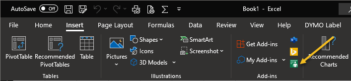
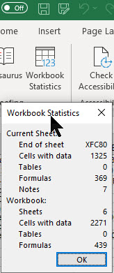
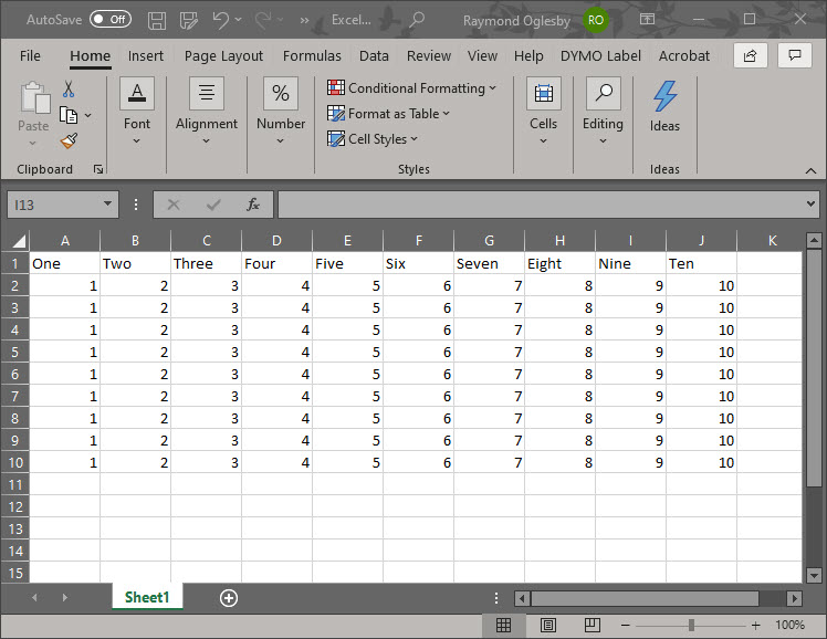
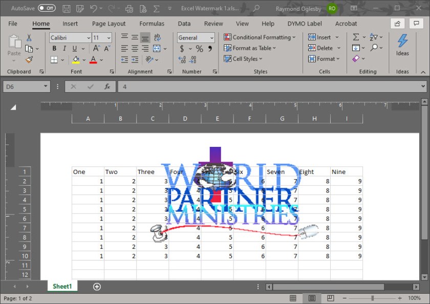
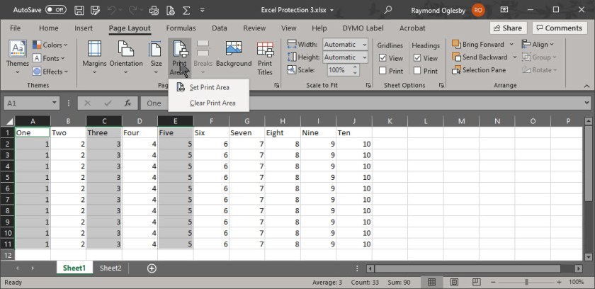
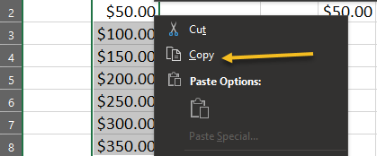
First, open Microsoft Excel. To copy, you can press Ctrl+C or right-click and select Copy. Refer to below image:
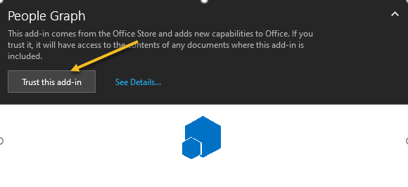
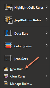
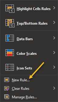
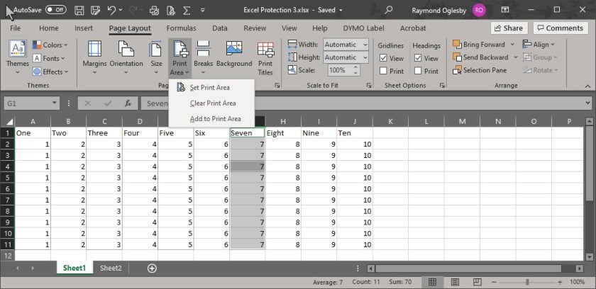
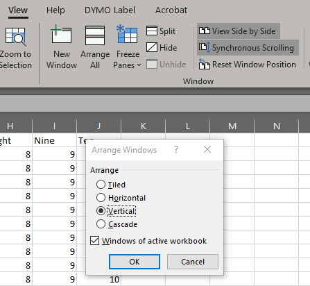
Now, do one of the following to access Paste Special.
- Click the Paste drop-down arrow in the ribbon on the Home tab, then select Paste Special.
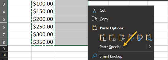
- Right-click cells that you are pasting to and select Paste Special in the shortcut menu.
See below image:
Use Simple Calculations With Paste Special
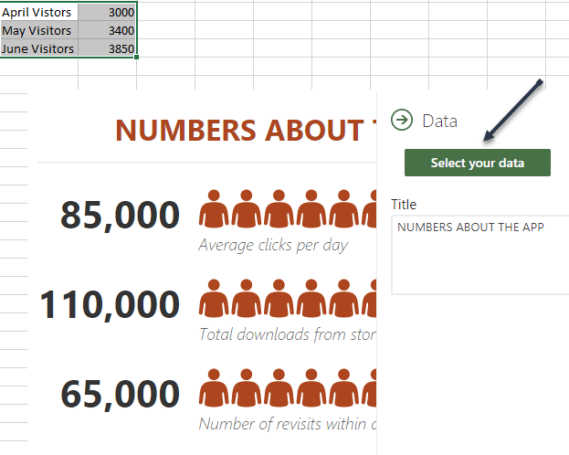
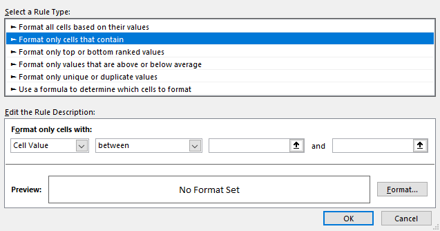
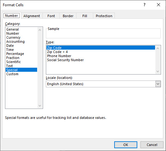
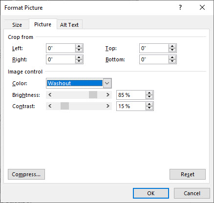
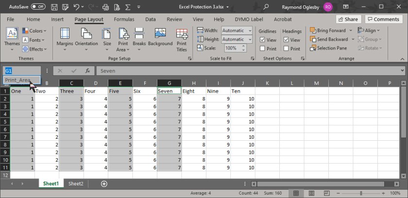
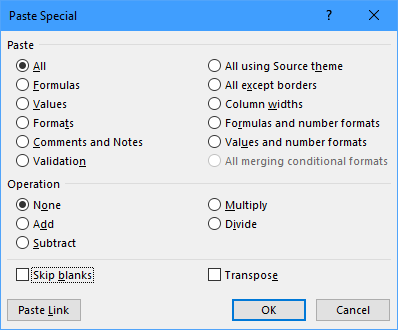
For basic numbers, decimals, and currency, you can choose from All, Values, or Values and Number Formats in the Paste section of the window. Use the best option for your data.
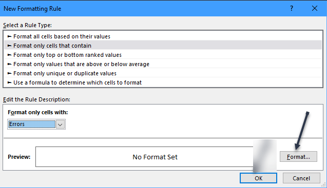
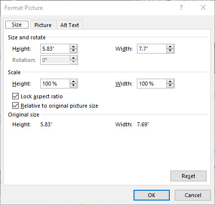
Next. you will use the section labeled Operation to add, subtract, multiply, or divide. See following image:
Let’s look at a simple example of one operation to see how it all works.
Add With Paste Special
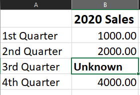
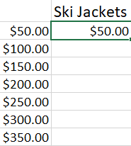
For this example, we want to add $50 to each of the amounts for our ski jacket prices to accommodate an increase.
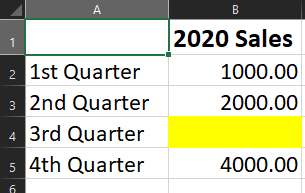
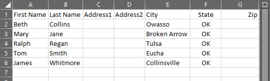
We enter $50 into a cell outside of our data set and copy it. You might already have the data in your sheet or workbook that you need to copy. Refer to below image:
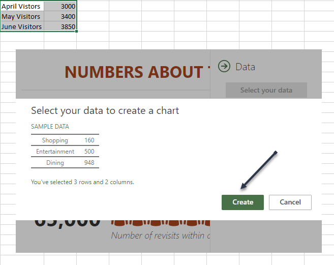
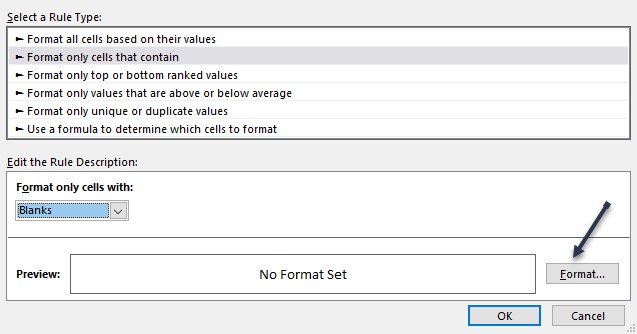
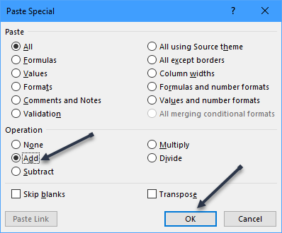
Now, we select the cells that we want to add $50 to and access Paste Special as described. Next, we choose Add in the Operation section and click OK. See below image:
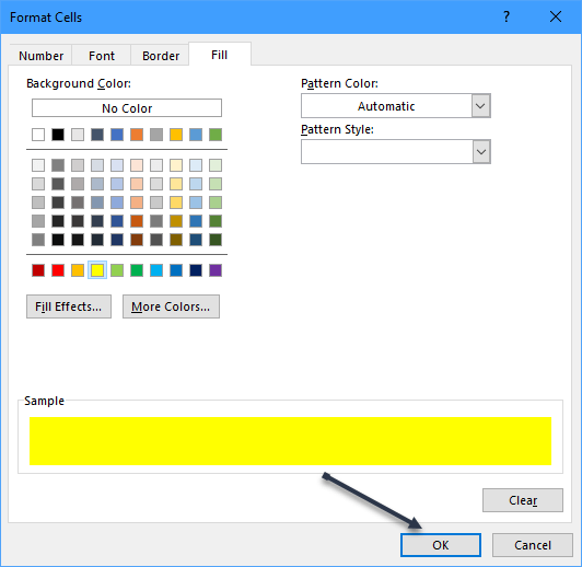
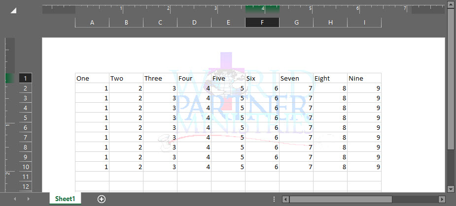
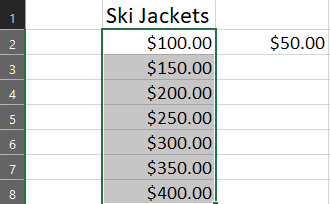
And that’s it. All of the cells in your selection have increased by $50. See following image:
Subtract, multiply, or divide an amount works the same way. For multiply or divide, you would use units instead of currency.
Be sure to switch the operation back to None when you are finished.
The next time you need to add, subtract, multiply, or divide a large group of cells in Excel by the same amount, remember this trick using Paste Special.
Quote For the Day
I’m sorry, if you were right, I’d agree with you.
Robin Williams
That’s it. Please feel free to share this post! One way to share is via Twitter.
Just click the Tweet icon below. This will launch Twitter where you click its icon to post the Tweet.
Check out TechSavvy.Life for blog posts on smartphones, PCs, and Macs! You may email us at contact@techsavvy.life for comments or questions.
Tweet
I Would Like to Hear From You
Please feel free to leave a comment. I would love hearing from you. Do you have a computer or smart device tech question? I will do my best to answer your inquiry. Just send an email to contact@techsavvy.life. Please mention the device, app and version that you are using. To help us out, you can send screenshots of your data related to your question.