How to Highlight Blank or Error Cells in Excel

RAYMOND OGLESBY @RaymondOglesby2
August 26, 2021

Spotting things in a spreadsheet can be much quicker when you highlight them. With conditional formatting in Microsoft Excel, you can make finding blank cells or formula errors easier. Let’s explore how this feature works.

This is for devices running Microsoft Excel

Highlight Blank Cells

When you have a spreadsheet full of data that you expect to fill every cell, you can easily overlook cells that are left empty.

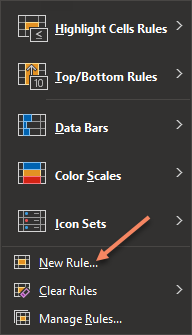
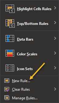
First, open the sheet and select the cells where you want to apply the formatting. Next, go to the Home tab and click Conditional Formatting in the Styles group of the Ribbon. Now, choose New Rule. Refer to below image:

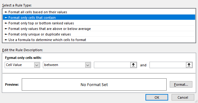
Next, in the New Formatting Rule window that appears, click Format only cells that contain under Select a Rule Type at the top. See below image:

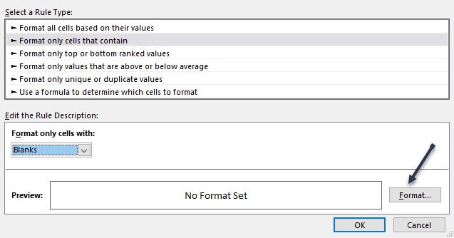
Now, at the bottom, pick Blanks in the Format only cells with drop-down box. Next, click Format to the lower right of the preview to select how to format the blank cells. See following image:

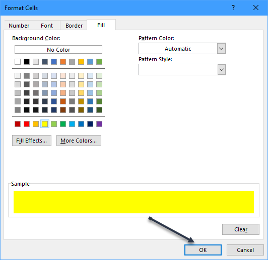
Now, in the Format Cells window, use the tabs at the top for Font, Border, and Fill to choose your formatting. Click OK. For our example, we are using Fill to color our blank cells bright yellow. Refer to below image:

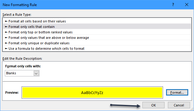
You will be back on the New Formatting Rule window, where you will see a preview of the formatting for blank cells. If you are happy with it, click OK to apply the conditional formatting. See below image:

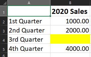
You should then see any empty cells in the range that you selected highlighted with the formatting that you picked. See following image:

Highlight Error Cells

Even though Microsoft Excel does a decent job of of pointing errors out to you, they might not be noticeable if you have a large sheet to scroll through. To make sure that you see the errors quickly, conditional formatting is the way to go.

You will actually follow the same process that you used in the previous section to highlight blanks, but with one difference.

First, switch to the Home tab, click Conditional Formatting, and then choose New Rule. Refer to below image:

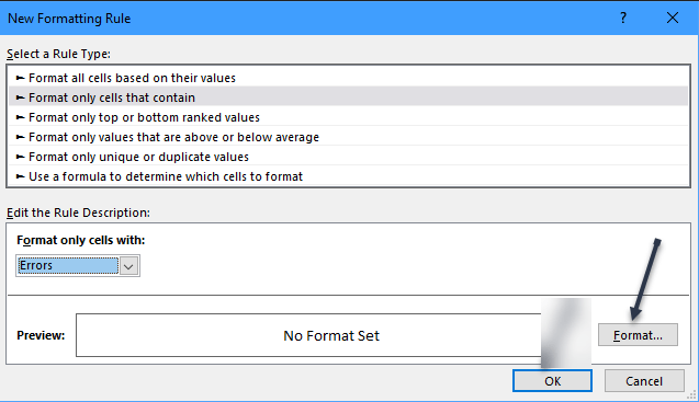
Next, in the New Formatting Rule window, pick Format only cells that contain at the top. But this time, pick Errors in the Format only cells with drop-down box at the bottom. Now, click Format to choose the formatting. See below image:

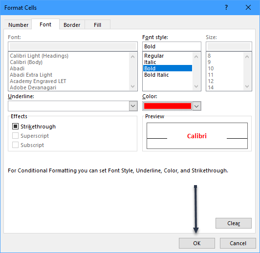
For this example, adjust the Font options to make the cells with errors bold and red. Click OK. After you pick the formatting, click OK again to apply the rule. See following image:

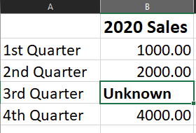
Now, those errors will be very visible! Refer to below image:

Quote For the Day

The true delight is in the finding out rather than in the knowing

Isaac Asimov

You are finished. Please feel free to share this post! One way to share is via Twitter.

Just click the Tweet icon below. This will launch Twitter where you click its icon to post the Tweet.

Check out TechSavvy.Life for blog posts on smartphones, PCs, and Macs! You may email us at contact@techsavvy.life for comments or questions.

Tweet

I Would Like to Hear From You

Please feel free to leave a comment. I would love hearing from you. Do you have a computer or smart device tech question? I will do my best to answer your inquiry. Just send an email to contact@techsavvy.life. Please mention the device, app and version that you are using. To help us out, you can send screenshots of your data related to your question.